
Neural Networks
Scroll to Learn!
What are Neural Networks?
A neural network is a machine learning model that is structured and operates much like the human brain. It's a system of interconnected nodes, or "neurons," organized in layers that process information. The primary goal of a neural network is to learn from data, identify complex patterns, and make predictions or classifications without being explicitly programmed for every single task.
Why Neural Networks are Unique
Neural networks are particularly powerful because they can learn and model intricate, non-linear relationships in data that are too complex for traditional algorithms to handle. This ability to approximate almost any function has made them the foundation of deep learning. They've been a key driver behind many of the most impressive AI breakthroughs in recent years.
Because of this power, neural networks excel at tasks that require understanding subtle patterns and context, such as:
-
Image Recognition: Identifying and classifying objects, faces, or scenes in a photograph. This is how your phone can automatically group photos of the same person or how a self-driving car "sees" the road.
-
Natural Language Processing (NLP): Understanding, generating, and translating human language. This technology powers chatbots, voice assistants like Siri and Alexa, and services that summarize long articles.
-
Recommendation Systems: Predicting what products, movies, or songs a user might like based on their past behavior and preferences. Platforms like Netflix and Spotify use neural networks to provide personalized suggestions.
Neural Network Architecture
Neural networks are named for mimicking the human brain with their system of interconnected neurons. Neural networks are fundamentally equations in which the coefficients (called weights or parameters) and constants (called biases) are modified so that the inputs (features in ML) and outputs (predictions of model) fit the pattern of the training data. Let's start by looking at single neurons.
The diagram represents what is known as a linear unit. It is a single neuron designed to perform simpler linear regression. It is composed of weight (w) which is the coefficient of its single feature (X). There is also a weight called a bias (b) which is the coefficient of 1 also known as a constant. The equation created by this neuron is ŷ=wx+b where the output of the neuron and in this case the prediction of the whole network is ŷ. During training w and b start at random values and are altered to so that the linear equation illustrates the pattern of the data.

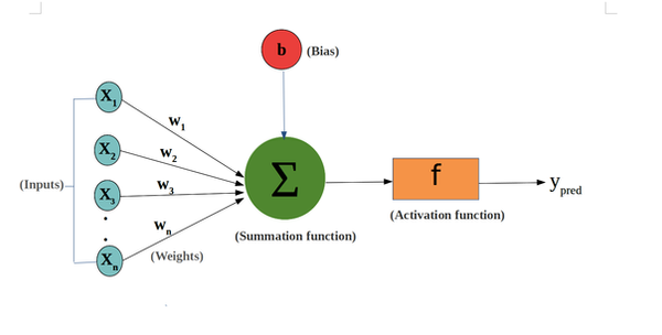
Let's take a look at something more complex and non linear. The neuron to the right has multiple inputs (features) and something new called an activation function denoted as f(x) which allows the model to learn complex non linear patterns. The equation for this neuron would be
a = f(w₁X₁+w₂X₂+w₃X₃...wₙXₙ+b)
or more concisely as follows, where 'a' is the output of the neuron.

Now Imagine many neurons feeding their a values forward to become one of the X values of another neuron until the final output layer. Each neuron has its own weights/biases and activation function. These combine to a long composite function that outputs the final prediction ŷ. The hidden layers add capacity to the model. A model with 3 or more hidden layers is known as a deep neural network or deep learning which can learn extremely sophisticated patterns

Neural Network Training
A neural network is trained with many iterations through the training dataset called epochs until the training is satisfactory. Each epoch, the following 4 step sequence is performed:
Step 1: Forward Pass
Inputs are passed in for training data. The Neural Network equation generates predictions and stores them.
Step 2: Loss Calculation
The Loss is calculated using a loss function (also known as a cost function). Different loss functions can be used but they all are based on the average absolute distance between the predicted and actual values for the training data. In this case we'll use a common one, mean squared error (MSE) as shown below

Understanding MSE:
Substituting the equation for ŷ which is in terms of a gives us a very long equation. Then substituting the values for a in gives us an even longer equation in which we can fill in all the values until the only values left are the weights and biases.
MSE makes graph in the muti-dimensional plane where the weights and biases are the horizontal axes and loss is the vertical axis. This can be visualized as a paraboloid in 3 dimensions when we have only one feature and one neuron as well as no activation function. However, with a more complex network this graph has more than 3 dimensions and thus cannot be visualized. Additionally it may not be perfectly bowl shaped but instead have many ruts or local minima.

Here is MSE plotted with the weight and bias on the horizontal axis and loss on the vertical axis
Step 3: Backpropagation
At this point the mathematical equations can get very complicated but ultimately Backpropagation is an algorithm that uses the chain rule in calculus (a rule for computing derivatives of composite functions like MSE) to calculate the partial derivative of each weight or bias with respect to loss. This is important because it determines the rate at which a change in each weight or bias will affect the loss. This essentially tells the model how to modify each weight and bias to minimize loss. By combining all of these partial derivatives into a single vector we get what is known as a gradient in multivariable calculus. This gradient represents the direction of steepest ascent. To visualize this think back to the bowl shaped graph and imagine you are standing at halfway to the bottom. The gradient vector shows the direction within the horizontal plane that you must travel to encounter the steepest vertical ascent. By traveling in the opposite direction you encounter the steepest downward descent, or in other words the quickest route to minimizing the loss by adjusting weights and biases


Step 4: Gradient Descent
Now that the gradient has been calculated we simply adjust all the weights accordingly each epoch to minimize loss. We use the following equation to do this:

Here the alpha symbol is the hyperparameter learning rate or the rate at which the weights are altered. If we have a high learning rate, the weights will be altered with greater magnitude. An excessively large learning rate may struggle to converge, bouncing around many times. An excessively small learning rate will take a very long time to converge due to only changing in small increments each iteration. In the case of complex patterns in data the loss function will have many local minima. Smaller learning rates have a tendency to converge into smaller minima and stop training because the gradient has reached zero. This prevents them from reaching the deepest global minima. On the other hand large learning rates may jump out and are more likely to converge in a deeper minima.

Like any hyperparameter, learning rate must be tuned and optimized to find the sweet spot for best results.
Most algorithms for training Neural Networks stem from something called Mini-Batch Stochastic Gradient Descent. Let's understand what this is.
Batch/Pure Gradient Descent: calculates the gradient of the cost function using the entire training dataset for each epoch
-
Pros:
-
Leads to a more stable and accurate gradient calculation, as it uses all data
-
Guarantees convergence to the global minimum for bowl shaped loss functions
-
-
Cons:
-
Computationally very expensive and slow for large datasets, requires more memory
-
More likely to get stuck in local minima for complex loss functions
-
Pure Stochastic Gradient Descent: calculates the gradient and updates the model's parameters using a single, randomly selected training example for each epoch.
-
Pros:
-
Significantly faster than batch gradient descent, especially for large datasets
-
The "noisy" updates from using random single examples can help it escape local minima in complex loss functions
-
-
Cons:
-
The updates are very noisy, causing the loss to fluctuate widely
-
Convergence is not as stable as with batch gradient descent; it jitters around the minimum instead of converging directly
-
Mini-batch Stochastic Gradient Descent is a compromise between the two extremes. Each epoch, it calculates the gradient and updates parameters using a small, randomly selected subset of the data called a mini-batch. This combines both techniques and is the most common form of gradient descent used in practice.
-
Pros:
-
More stable than stochastic gradient descent and thus better than converging
-
Still random unlike pure gradient descent and thus better at jumping out of local minima
-
Not as slow as pure gradient descent
-
The use of mini-batches allows for parallel processing on GPUs, which speeds up training.
-
-
Cons:
-
Requires the user to choose a hyperparameter: the mini-batch size
-
The updates are still noisier than batch gradient descent
-
Still not as fast as stochastic gradient descent
-
When the training loss either reach zero or stops improving significantly after each successive epoch, training is ends. You have officially covered all of the basic steps of training a neural network!
Convolutional Neural
Networks
So far we've only talked about the most traditional type of neural networks, feedforward networks. These are great for simple tasks like classification and regression of standard spreadsheet style data. Let's look at some other types of neural networks with their own unique purposes.
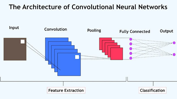
A convolutional neural network (CNN) is a specialized type of deep learning model that excels at processing grid-like data, such as images. Unlike traditional neural networks that treat every input (like a pixel) independently, CNNs leverage the spatial relationships between data points, making them highly effective for computer vision tasks in which the model must analyze image data. For perspective, some examples of computer vision technologies include facial recognition, self-driving cars, or the detection of diseases from medical imaging.
CNNs are composed of 3 specialized types of layers:
-
Convolutional Layer: This layer uses filters to scan the input data (e.g., an image) and extract key features like edges, textures, and shapes.
-
Pooling Layer: This layer reduces the size of the data while keeping the most important information, making the network more efficient and preventing overfitting.
-
Fully Connected Layer: The final layers take the features extracted by the previous layers and use them for classification or prediction.
Recurrent Neural
Networks
A recurrent neural network (RNN) is a type of neural network that's designed to process sequential data, like text or time series. Unlike traditional neural networks, which treat each input as independent, RNNs have a built-in "memory" that allows them to use information from previous steps in the sequence to influence the output of the current step.
This is done through a recurrent connection, where the output of a hidden layer is fed back into itself along with the new input at each time step. This feedback loop enables the network to maintain an internal state, or memory, that captures information about the past data it has processed.
RNNs and their variants are widely used for tasks that involve sequential data, including:
-
Natural Language Processing (NLP): Tasks like machine translation (e.g., Google Translate), sentiment analysis, and text generation.
-
Speech Recognition: Converting spoken words into text (e.g., voice assistants like Siri and Alexa).
-
Time Series Forecasting: Predicting future values based on historical data, such as stock prices or weather patterns.
-
Image Captioning: Generating a descriptive sentence for an image by combining a convolutional neural network (CNN) with an RNN.
Limitations & Variants
A major challenge for basic RNNs is the vanishing gradient problem, which makes it difficult for them to learn long-term dependencies. As information passes through many time steps, the gradient (the signal that helps the network learn) can become so small that the network effectively "forgets" information from earlier in the sequence.

Long Short Term Memory
Long Short-Term Memory (LSTM) is a specific type of recurrent neural network (RNN) that is designed to solve the vanishing gradient problem that plagues standard RNNs. This problem makes it difficult for traditional RNNs to learn and remember information from earlier in a long sequence of data, effectively giving them a very short-term memory. LSTMs overcome this by using a more complex internal structure that allows them to selectively remember or forget information over long periods.
Instead of a single recurrent connection, an LSTM has a more sophisticated internal "cell" with multiple gates that regulate the flow of information. This cell acts like a memory unit and has a dedicated path for information to flow through without being altered, which prevents the vanishing gradient problem. The three main gates are:
-
Forget Gate: This gate decides what information from the previous state should be thrown away because it's no longer relevant.
-
Input Gate: This gate determines what new information from the current input should be stored in the cell state.
-
Output Gate: This gate controls which parts of the cell state will be used as the output for the current time step and passed on to the next one.
By controlling the flow of information with these gates, LSTMs can maintain a "long-term memory" (the cell state) while also having a "short-term memory" (the hidden state) that can be easily updated.
